These are the figures and tables of the revised manuscript, with their captions, shared with the editor
and the referees during the discussion. If anything here differs from the revised manuscript as submitted, the revised
manuscript prevails.
Figure and table numbers here are those of the revised manuscript; the author comments use those of the
discussion paper. Tables 2 to 4 are Tables 1 to 3 of the discussion paper, and Tables 1, 5 and 6 are new. Figures 1 to
10, A1 and A2 keep their numbers; Figs. A3 and A4 are new and take the place of Figs. A4 and A5 of the discussion paper,
and Fig. A3 of the discussion paper is removed.
Updated on 1 November 2026: Fig. 7 is redrawn with the eight-neighbor boundary test; the table of Fig. 3(b)
and its caption give regions 10001 and 10002 west of the antimeridian; and the captions of Figs. 5(f), 6 and 7
are corrected, as in the revised manuscript; see CHANGES.txt.
Files: each figure as PNG and PDF, each table as CSV, the Python script that draws each figure
(links under each item), and the input data of the scripts as one zip (fullbasin-figure-data.zip, 122.4 MB); see
README.txt.
Main text: figures
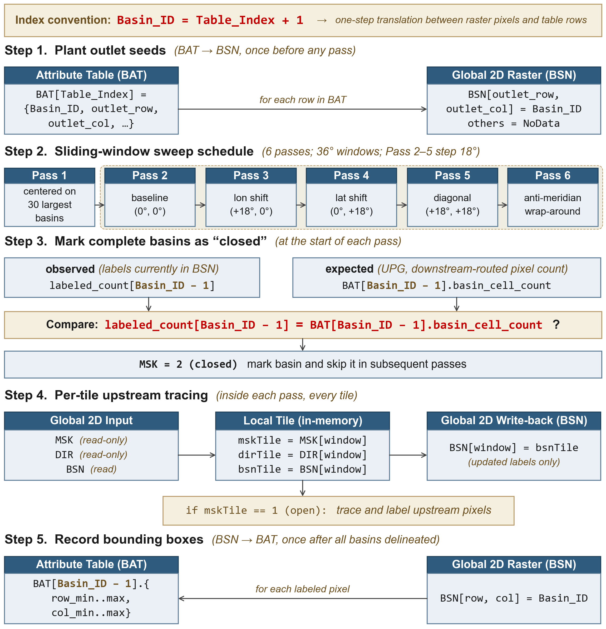
Figure 1. Schematic of the seamless global delineation framework, organized as five steps. Step 1 plants outlet seeds: for each row in the Basin Attribute Table (BAT), the outlet pixel in the global raster (BSN) is set to its Basin_ID under the index convention Basin_ID = Table_Index + 1 (Eq. (1)), and all other land pixels are set to NoData. Step 2 specifies a sliding-window sweep schedule of six 36° passes: Pass 1 centers windows on the 30 largest basins; Passes 2–5 step by 18° in longitude, latitude, and the diagonal from a (0°, 0°) baseline; Pass 6 wraps the antimeridian. Step 3 marks complete basins as closed at the start of each pass: the observed labeled_count[Basin_ID − 1] from BSN is compared against the expected BAT[Basin_ID − 1].basin_cell_count (the UPG pixel count at the outlet); on equality (Eq. (2)) the basin’s mask is set to MSK = 2 (closed) and skipped in subsequent passes. Step 4 traces upstream per tile inside each window: read-only globals MSK, DIR, and BSN are buffered into local tiles mskTile, dirTile, bsnTile; for pixels with mskTile == 1 (open), upstream pixels are traced and labeled; updated labels in bsnTile are written back into the global BSN. Step 5 records bounding boxes once all basins are delineated: BSN is scanned and per-basin row/column extents are written back to BAT as row_min..max, col_min..max.
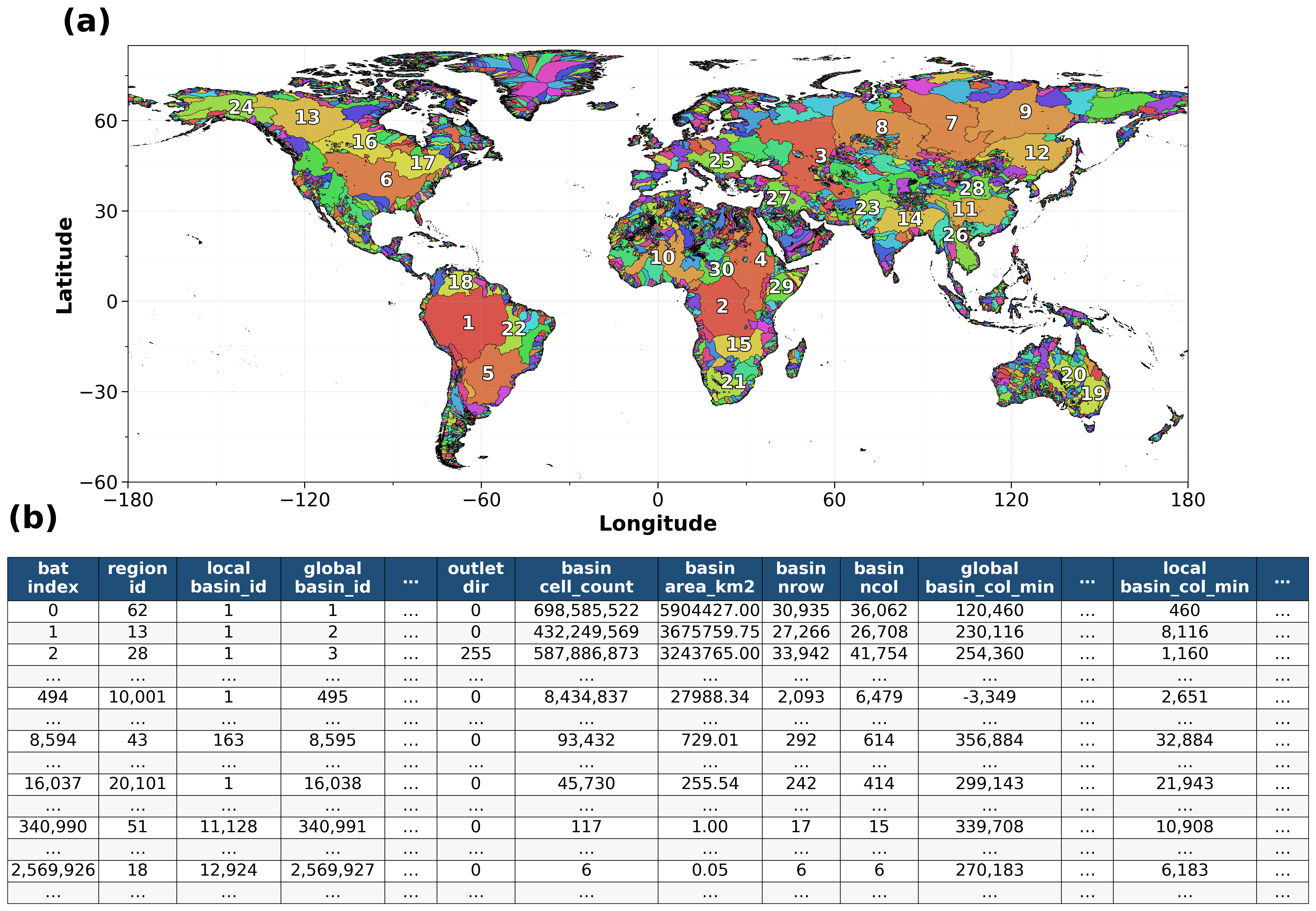
Figure 2. Global basin mask and Basin Attribute Table. (a) Global basin mask (BSN); basins are colored by global_basin_id from a cycle of 100 colors, so a color can recur. The 30 largest basins, ranked by drainage area, are labeled for reference. (b) Structure and example records of the Basin Attribute Table (BAT). Key fields include the triple linking key (global_basin_id, region_id, local_basin_id), outlet attributes (drainage destination, pixel count, and upstream drainage area), basin footprint dimensions (number of rows and columns), and spatial bounding box indices on both the global and regional grids; region_id and the regional fields refer to the 90 processing regions of Fig. 3. The complete BAT contains 24,587,290 outlet records. Of these, 8,888,059 are single-pixel outlets, mostly along coastlines, where a pixel drains directly to the ocean with no upstream pixel, and a further 13,129,317 drain at least two pixels but less than 0.05 km²; all are retained in the BAT for completeness. For global_basin_id = 495, the global bounding box extends across the 180° E/W antimeridian. For global_basin_id = 3, the outlet_dir equals 255, indicating an endorheic (internally draining) basin (the Caspian Basin, approximately 3.24 million km²).
Figure 3. Global processing regions and Regional Attribute Table. (a) Global region mask (RGN) showing the 90 processing regions. The 65 continental regions follow the HydroBASINS Level-02 units (Lehner and Grill, 2013): 57 carry the two-digit Level-02 code, and 8 four-digit regions divide a unit with too many pixels for a 32-bit index along its Level-03 units, the identifier naming the first and last units held (e.g., region 5618 holds units 561–568). Two antimeridian regions (IDs 10001–10002) group basins that cross the 180° E/W antimeridian, and 23 island-group regions (IDs 20101–20901) consolidate isolated island basins by spatial proximity. (b) Structure and example entries of the Regional Attribute Table (RAT), listing spatial bounding indices (region_row_min/max and region_col_min/max), region dimensions (region_nrow and region_ncol), and the number of valid land pixels (region_grid_count) within each bounding box. For region 10001, the negative region_col_min (−6,000) reflects the bounding box extending west of the antimeridian. The tiles of regions 10001 and 10002 are georeferenced 360° east of their RAT longitudes. All regional bounding boxes are snapped to integer-degree boundaries (multiples of 1,200 pixels at 3 arcsec resolution) to ensure exact alignment with global rasters.
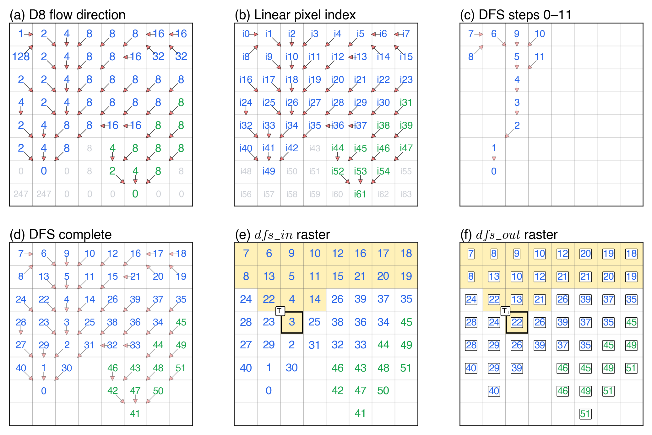
Figure 4. Schematic of the flow-tree index on an 8 × 8 D8 flow-direction raster containing two basins: Basin A (blue, 41 pixels) and Basin B (green, 11 pixels). Pixels are numbered once each, in the depth-first order of the flow tree (Tarjan, 1972), as in the modified nested set model (Haag and Shokoufandeh, 2019) that Haag et al. (2018) applied to D8 grids; children are sorted by upstream drainage area (UPA) in descending order so that the main stem is numbered first. (a) D8 flow-direction codes with arrows indicating flow paths. (b) Linear pixel indices (i0–i63); gray labels mark invalid pixels. (c) A snapshot after steps 0–11: arrows and numbers appear only for pixels visited so far; each number is the entry order dfs_in. (d) The completed traversal, numbering all 52 valid pixels from 0 to 51. (e) The final dfs_in raster. (f) The final dfs_out raster: dfs_out is the largest dfs_in among the pixels upstream of a pixel, the pixel included, and equals dfs_in + upg − 1 (Fig. A3). Light yellow marks the 20 pixels upstream of T₁ = i26, whose interval is [3, 22].
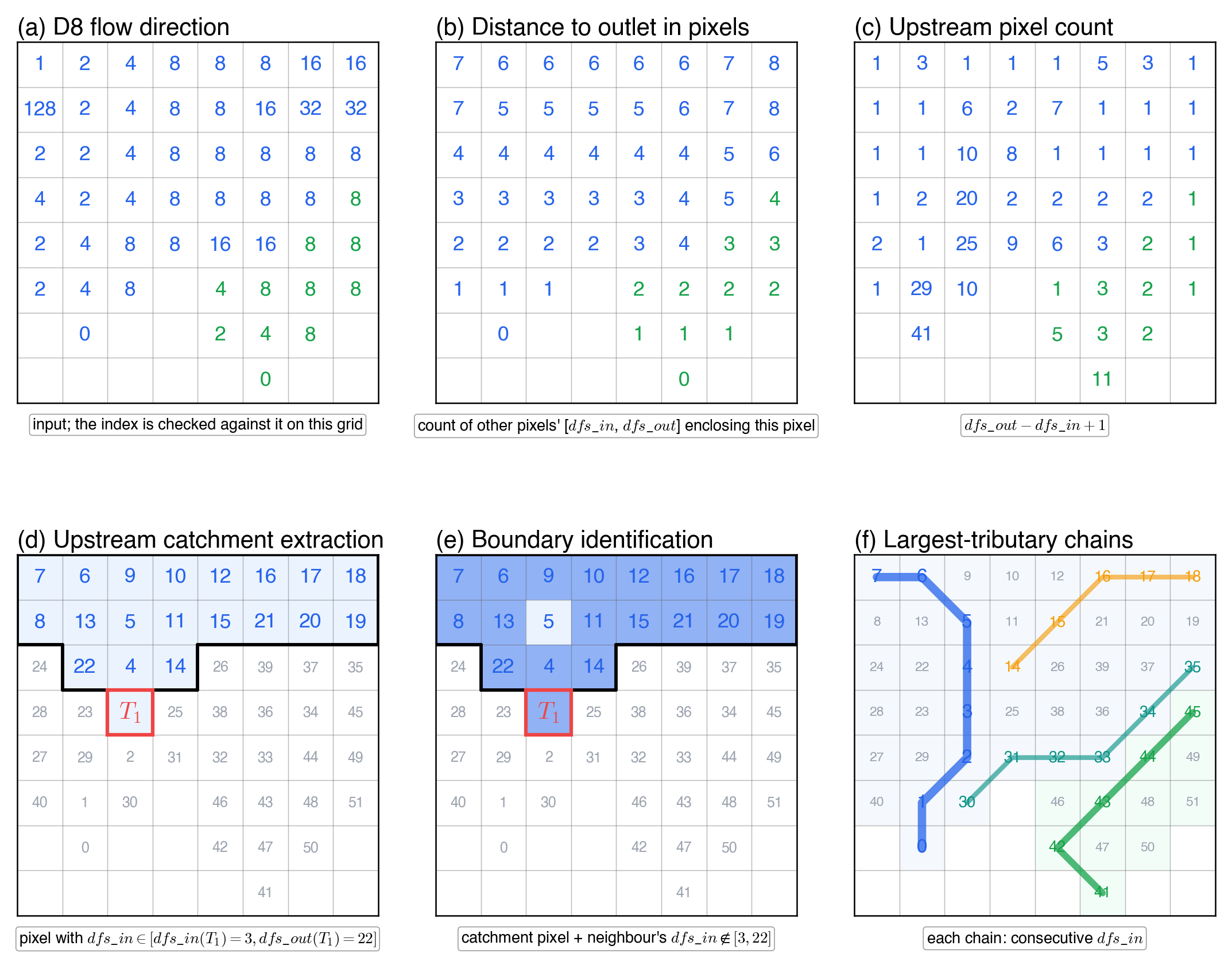
Figure 5. Capabilities of the flow-tree index, illustrated on the 8 × 8 example grid of Fig. 4. (a) The input D8 flow direction; the index is checked against it at every pixel. (b) The distance to the outlet in pixels, equal to the number of other pixels whose interval [dfs_in, dfs_out] encloses the pixel. (c) The upstream pixel count, dfs_out − dfs_in + 1. Panels (d) and (e) take T₁ = pixel i26 in Basin A, with [dfs_in, dfs_out] = [3, 22], as the example target: (d) the upstream catchment of T₁, the pixels whose dfs_in lies in [3, 22] (interval test), with the 4-connected boundary drawn in black; (e) the catchment boundary, the catchment pixels with at least one neighbor whose dfs_in lies outside [3, 22]. (f) Largest-tributary chains in both basins, each occupying consecutive dfs_in values (Eq. (6); blue: Basin A’s main stem, 0–7; teal, 30–35, and orange, 14–18: two of its tributaries; green: Basin B’s main stem, 41–45).
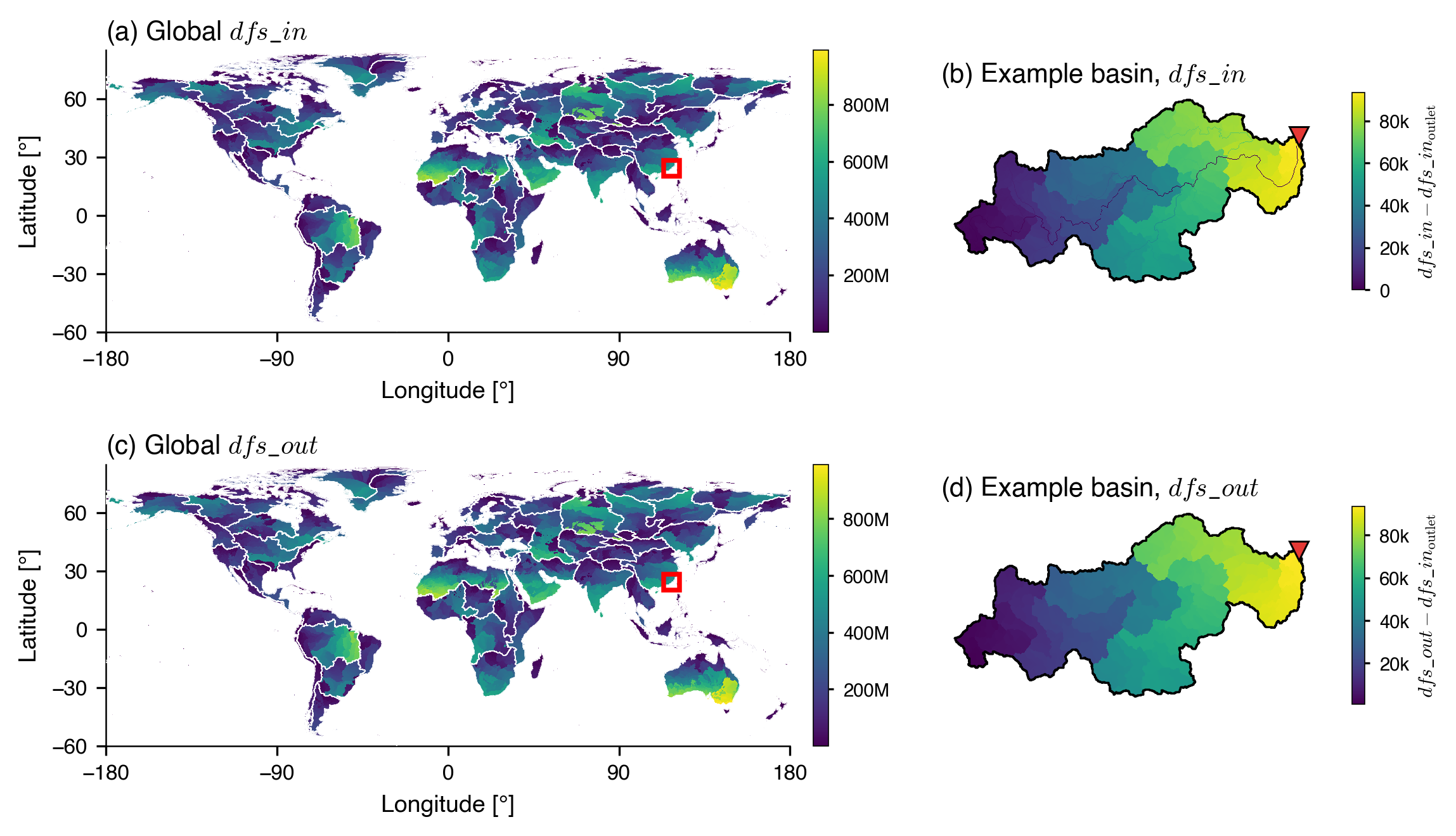
Figure 6. Global flow-tree index of FullBasin with a zoom into the example basin. The pixels of each of the 90 regions are numbered from 0, one number per pixel. (a, c) dfs_in and dfs_out sampled at one pixel per 1/20° (the center pixel of each 60 × 60 block) and displayed at 1/10°; thin white lines trace the region boundaries. Because sibling branches are numbered in descending order of upstream drainage area, consecutive dfs_in values trace each basin’s main stem before branching outward into tributaries, and the spatial pattern of dfs_in visually recovers the river network. The red rectangle locates the example basin (basin 8595, 729 km², southeastern Fujian, China). (b, d) Zoom-in on the example basin at the native 3 arcsec resolution showing dfs_in and dfs_out, each minus the dfs_in of the outlet: 0–93,431 in (b) and 948–93,431 in (d); the black polygon traces the basin boundary and the red triangle (▼) marks the outlet (117.91° E, 24.40° N). dfs_out is computed from dfs_in and upg (Fig. A3). Each panel uses an independent viridis color scale.
Figure 7. Boundary walk on the example basin (basin 8595, southeastern Fujian, China; 729 km², 3 arcsec resolution). All four panels share the same dfs_in color fill, basin perimeter (black), stream polylines (white; UPA ≥ 10 km²), and outlet marker (▼). (a) For a target T₁ on the main stem, the boundary of upstream(T₁) is identified by the eight-neighbor interval test, two comparisons per candidate; the part on the basin perimeter is shown in gray, and the closing edge inside the basin in red. (b) Moving the target downstream to T₂, the new ring is derived from the previous ring by symmetric difference: pixels common to Boundary(T₁) and Boundary(T₂) (gray), pixels deleted when T₁ → T₂ (red), and pixels added at T₂ (green). (c) The 20 branch tips S₁…S₂₀ of the basin. The main stem S₂₀ follows the larger upstream area at every confluence; the other tips are ordered upstream-first by the position of their junction along the main stem. Black arrows indicate the downstream flow direction at each tip. (d) Splitting the main stem at 33 % and 67 % of its pixels yields two additional sub-streams S₂₁ and S₂₂ (blue), demonstrating intra-basin parallelism for the boundary walk.
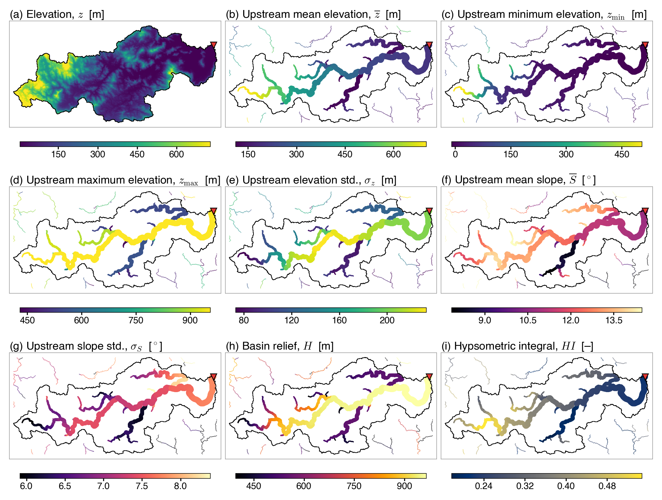
Figure 8. Per-pixel upstream terrain attributes of the example basin (global_basin_id = 8595; local_basin_id = 163; 729 km², southeastern Fujian, China): (a) elevation z (MERIT DEM v1.0.3, shown for context), (b) upstream mean elevation z̄, (c) upstream minimum elevation zmin, (d) upstream maximum elevation zmax, (e) upstream elevation standard deviation σz, (f) upstream mean slope S̄, (g) upstream slope standard deviation σS, (h) basin relief H, and (i) hypsometric integral HI. Panels (b)–(g) are the six upstream aggregates in Table 4, with means and standard deviations weighted by pixel area; (h) and (i) are the two arithmetic derivatives, computed pixel-wise from (b)–(d). Each target pixel (UPA ≥ 10 km²) is drawn as a filled circle whose radius scales with log10(UPA), so main-stem pixels appear larger. Pixels from neighboring basins sharing the bounding box are plotted at a uniform small radius with 50 % opacity for geographic context. Color bars are clipped at the 2nd and 98th percentiles. The black polygon traces the basin boundary; the red triangle (▼) marks the outlet.
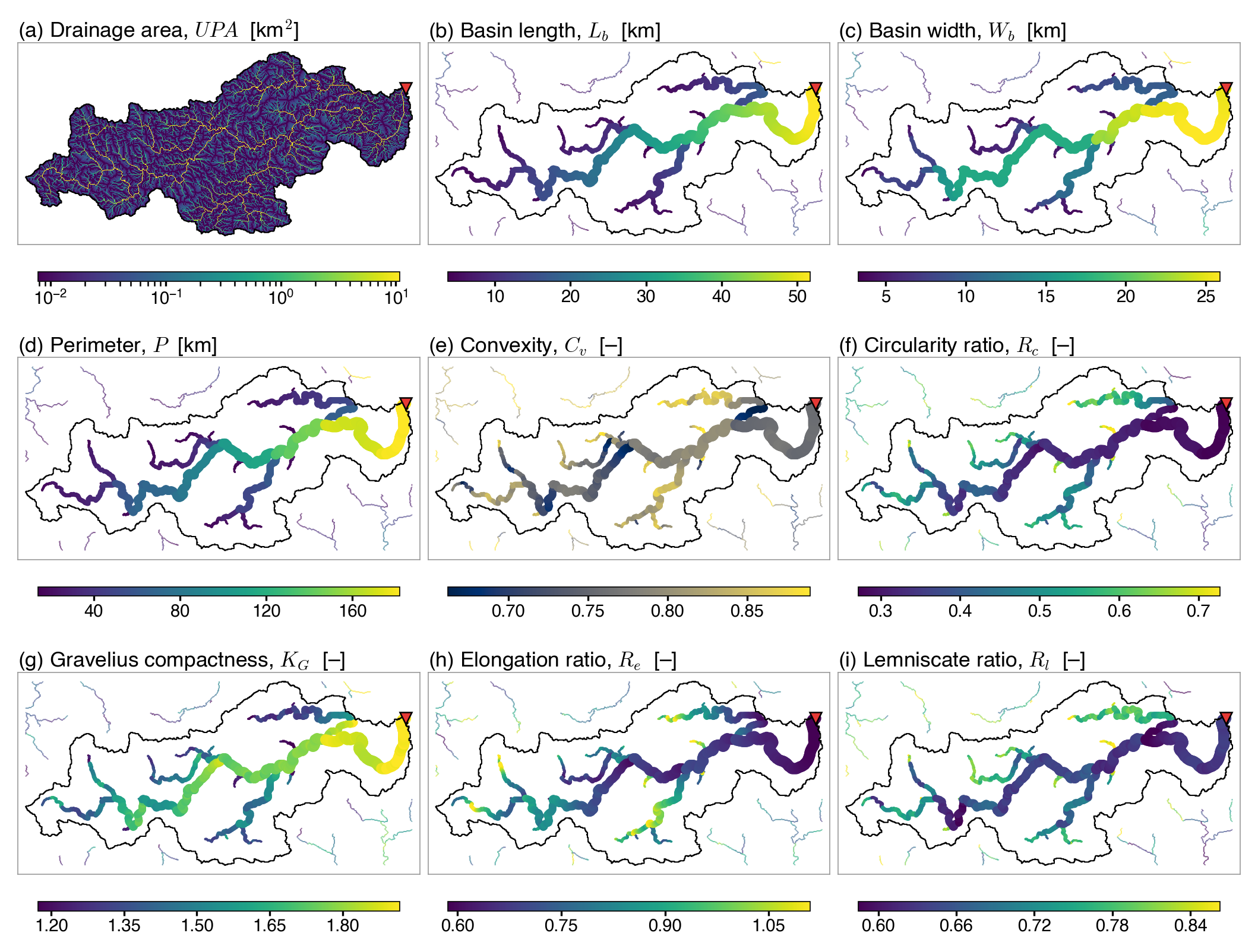
Figure 9. Per-pixel planform and shape attributes of the example basin (global_basin_id = 8595; local_basin_id = 163; 729 km², southeastern Fujian, China): (a) drainage area UPA at every pixel (shown for context), (b) basin length Lb, (c) basin width Wb, (d) perimeter P, (e) convexity Cv, (f) circularity ratio Rc, (g) Gravelius compactness KG, (h) elongation ratio Re, and (i) lemniscate ratio Rl = Pl/P, where Pl is the perimeter of the ideal lemniscate with area A and length Lb (Chorley et al., 1957). Panels (b)–(e) are the four boundary-walk metrics in Table 4, traced on each target’s upstream-catchment outline, with lengths measured along great circles; panels (f)–(i) are the four dimensionless shape ratios, computed pixel-wise from panels (a), (b), and (d). Each target pixel (UPA ≥ 10 km²) is drawn as a filled circle whose radius scales with log10(UPA), so main-stem pixels appear larger. Pixels from neighboring basins sharing the bounding box are plotted at a uniform small radius with 50 % opacity for geographic context. Color bars are clipped at the 2nd and 98th percentiles. The black polygon traces the basin boundary; the red triangle (▼) marks the outlet.
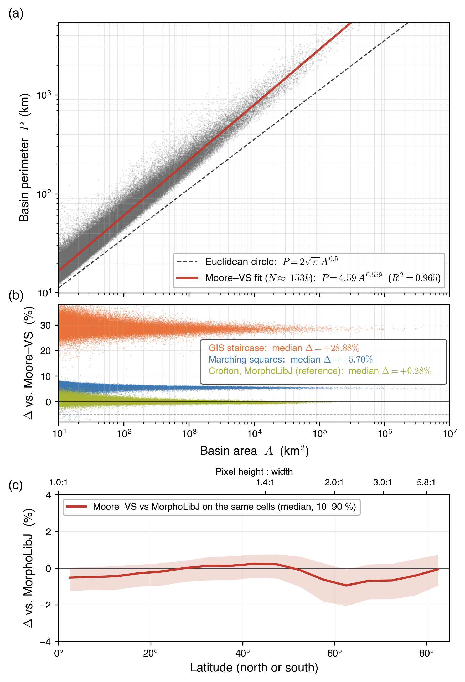
Figure 10. Perimeter–area scaling and cross-validation of the released Moore–VS perimeter on 153,196 global records (outlet + sub-mid, A ≥ 10 km²). (a) Log-log scatter of basin perimeter P against area A, with the Moore–VS power-law fit P = 4.59 · A0.559 (R² = 0.965) and the circle reference P = 2√π · A0.5 (dashed). The exponent exceeds 0.5, consistent with the fractal character of drainage divides (Mandelbrot, 1967). (b) Relative deviation Δ = 100 × (Pmethod − PMoore–VS)/PMoore–VS versus A for three other methods: GIS staircase (median +28.88 %) and marching squares (median +5.70 %), both for pixel aspect ≤ 1.2 (66,467 records, within about 34° of the equator); and the Crofton perimeter of MorphoLibJ (Legland et al., 2016), the reference, at all latitudes on the same cells as Moore–VS (152,468 records; median +0.28 %, 2nd–98th percentiles −0.89 % to +2.06 %). Reference lines mark Δ = 0 and ±5 %. (c) Δ = 100 × (PMoore–VS − PMorphoLibJ)/PMorphoLibJ on the same cells, by latitude: median and 10–90 % range per 5° band (overall median −0.28 %, 10–90 %: −1.24 % to +0.50 %; band medians from −0.94 % at 60–65° to +0.24 % at 40–45°); the top axis gives the pixel height-to-width ratio. MorphoLibJ serves as a reference, not as truth. Appendix B describes the methods.
D8 flow-direction raster of MERIT Hydro; code 0 marks an outlet at the coast (exorheic), 255 an inland sink (endorheic), and 247 no data.
UPG (upg)
Upstream pixel count of MERIT Hydro, derived from DIR; it counts the pixel itself.
UPA
Upstream drainage area of MERIT Hydro, in km², derived from DIR.
BSN
Basin-ID raster: each land pixel holds the global_basin_id of the outlet it drains to.
RGN
Region-ID raster: each land pixel holds the region_id of its region (90 regions).
BAT
Basin Attribute Table: one row per outlet (24,587,290 rows), with the position and type of the outlet, its pixel count and area, and its global and local bounding boxes.
RAT
Region Attribute Table: one row per region, with its bounding box and pixel counts.
MSK
Per-basin status mask used during delineation: before each window pass, the labelled pixel count of a basin is compared with its count in BAT (Eq. 2); MSK = 2 marks a closed basin, which later passes skip.
dfs_in
Number of a pixel in the depth-first order of the flow tree (Tarjan, 1972; Haag et al., 2018), from 0 to n − 1 over the n pixels of a region; the pixels upstream of p, p included, are numbered dfs_in(p) to dfs_out(p). Computed from seq_dfs and upg (Fig. A3).
dfs_out
dfs_in + upg − 1, the largest dfs_in among the pixels upstream of a pixel; computed, not released.
seq_dfs
The released layer of the flow-tree index (Table 2): the numbers dfs_in in reverse order within each basin, so that every pixel has a larger number than the pixels upstream of it and the outlet holds the largest number of its basin.
global_basin_id, region_id, local_basin_id
Triple key of a basin: its ID across the globe (1 to 24,587,290), the ID of its region, and its ID within the region (from 1).
target pixel
Pixel with at least 10 km² of upstream area, at which the sixteen attributes are given (436,633,884 pixels).
region tile
Raster of one region, cut from the global grid along the bounding box of the region, whose edges fall on multiples of 1,200 pixels of the global grid.
tier
One of the three parts of the dataset: basins and regions (tier 1), the flow-tree index (tier 2) and the sixteen upstream attributes (tier 3).
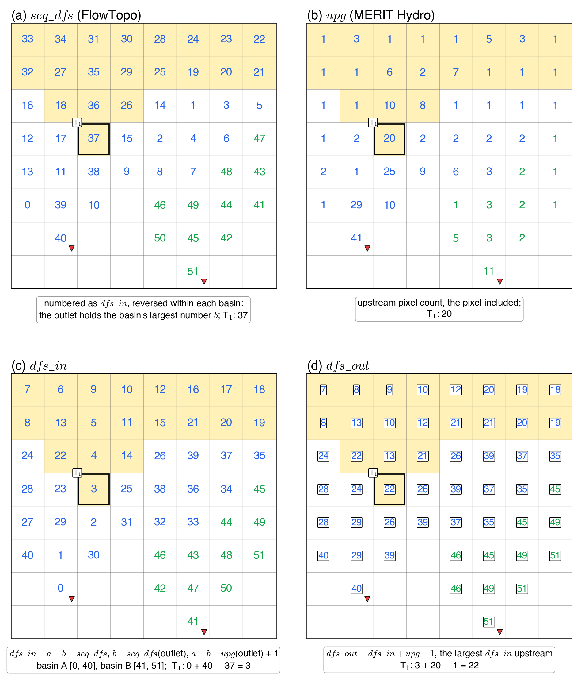
Table 2. Summary of input datasets and output products. All native-resolution rasters share a global grid (432,000 × 174,000 pixels of exactly 1/1200°) and are distributed as Cloud-Optimized GeoTIFF files with internal tiling; the ID rasters (basins, regions and basin groups) also carry overviews and color tables. Tabular products are in CSV and Apache Parquet format, and the outlines of the regions, the basin groups and the basins of 1 km² or more are also given as GeoPackage and GeoParquet polygons. The BAT and its per-region subsets share three linking keys (global_basin_id, region_id, local_basin_id) enabling direct cross-referencing between raster masks and attribute records. BAT and RAT column definitions are introduced where each field first appears in Sect. 3. File-name wildcard * denotes the region_id in six digits (e.g., seq_dfs_region_000011_90m.tif). The inputs are not redistributed; dfs_in and dfs_out are obtained from seq_dfs and upg. dfs_in is released in the form seq_dfs, which reverses dfs_in within each basin; dfs_in = a + b − seq_dfs, where b is the value at the basin outlet and a = b − upg(outlet) + 1 (Fig. A3).
File Name
Variable
Type
NoData
Inputs: MERIT Hydro v1.0.1 and MERIT DEM v1.0.3 (global coverage; not redistributed)
dir
Flow direction
—
—
upg
Upstream pixel count
—
—
upa
Upstream drainage area (km²)
—
—
dem
Elevation (MERIT DEM)
—
—
Basin and region masks with attribute tables (global coverage)
bsn_global_90m.tif
Basin mask
UInt32
0
rgn_global_90m.tif
Region mask
UInt16
0
bat_global_90m.csv, .parquet
Basin attribute table
—
—
rat_global_90m.csv, .parquet
Region attribute table
—
—
rgn_global.gpkg, .geo.parquet
Region outlines
—
—
Basin attribute tables and outlines (region tiles)
bat_region_*_90m.csv, .parquet
Basin attribute table
—
—
bsn_region_*_90m_gt1km2.gpkg, .geo.parquet
Basin outlines, basins of 1 km² or more
—
—
Basin groups, HydroBASINS Levels 1 to 3 (global coverage)
grp_global_90m_l{1,2,3}.tif
Basin-group mask
UInt32
0
gat_global_90m_l{1,2,3}.csv, .parquet
Group attribute table
—
—
grp_global_l{1,2,3}.gpkg, .geo.parquet
Group outlines
—
—
Flow-tree index (region tiles; released in the FullTopo record)
seq_dfs_region_*_90m.tif
Depth-first order within each basin, outlet last; gives dfs_in and dfs_out with upg (Fig. A3)
Table 3. Global outlet counts fully stratified by drainage destination (exorheic and endorheic), for all outlets and across six area thresholds (≥ 0.05, ≥ 1, ≥ 25, ≥ 100, ≥ 1,000, and ≥ 10,000 km²). No area threshold is applied in the delineation: the first column counts every outlet, down to single-pixel coastal outlets (0.001–0.009 km²).
Table 4. Sixteen per-pixel upstream morphometric attributes of FullBasin, delivered as GeoTIFF rasters at native 3 arcsec (approximately 90 m) resolution for targets with upstream drainage area ≥ 10 km². Attributes fall into three algorithmic classes: upstream aggregation and boundary walk are structural passes over the DFS-indexed flow tree, while arithmetic entries are pixel-wise combinations of preceding rasters. Elevation z is from MERIT DEM v1.0.3 and slope S is computed from it; ai is the area of pixel i. A is the upstream drainage area (UPA). Lengths are of great circles, taken on the WGS84 ellipsoid: d between two pixels, and projW, the signed perpendicular distance of a boundary pixel from the great circle of Lb; Aconvex hull is also taken on the ellipsoid. Pl is the perimeter of the ideal lemniscate with area A and length Lb. Classical references for each variable are listed in the rightmost column and discussed in Sect. 5. The corresponding raster filenames are listed in Table 2.
Table 5. What each type of query reads and how its cost scales. The index is numbered within each region and every basin lies in one region, so a pixel in another region is never upstream of p.
Query
What is read
Cost
Basin or region of a pixel; its record
one pixel of BSN or RGN; one row of BAT or RAT
constant
One of the sixteen upstream attributes at a pixel
one pixel of the attribute layer
constant
Is pixel q upstream of target p?
dfs_in(q), dfs_in(p), upg(p)
two comparisons
Upstream aggregate of a new variable, one target
the variable and dfs_in over the bounding box of p’s basin; upg(p)
linear in the box
Upstream aggregates of a new variable, many targets
the variable and dfs_in over the basin or region; upg at the targets
linear once (scatter and prefix sum), then two lookups per target
Table 6. The sixteen attributes of FullBasin over all pixels where they are given (436,633,884 pixels with at least 10 km² of upstream area; the hypsometric integral is absent at 9,212 pixels whose catchment has no relief, and the lemniscate ratio at 2,318 pixels whose k = πLb2/(4A) is below 1/2, for which the ideal lemniscate crosses itself): minimum, percentiles, maximum and mean. Attribute numbers (#) as in Table 4. The table, with the global row and column of each minimum and maximum, is also released with the data as a CSV file.
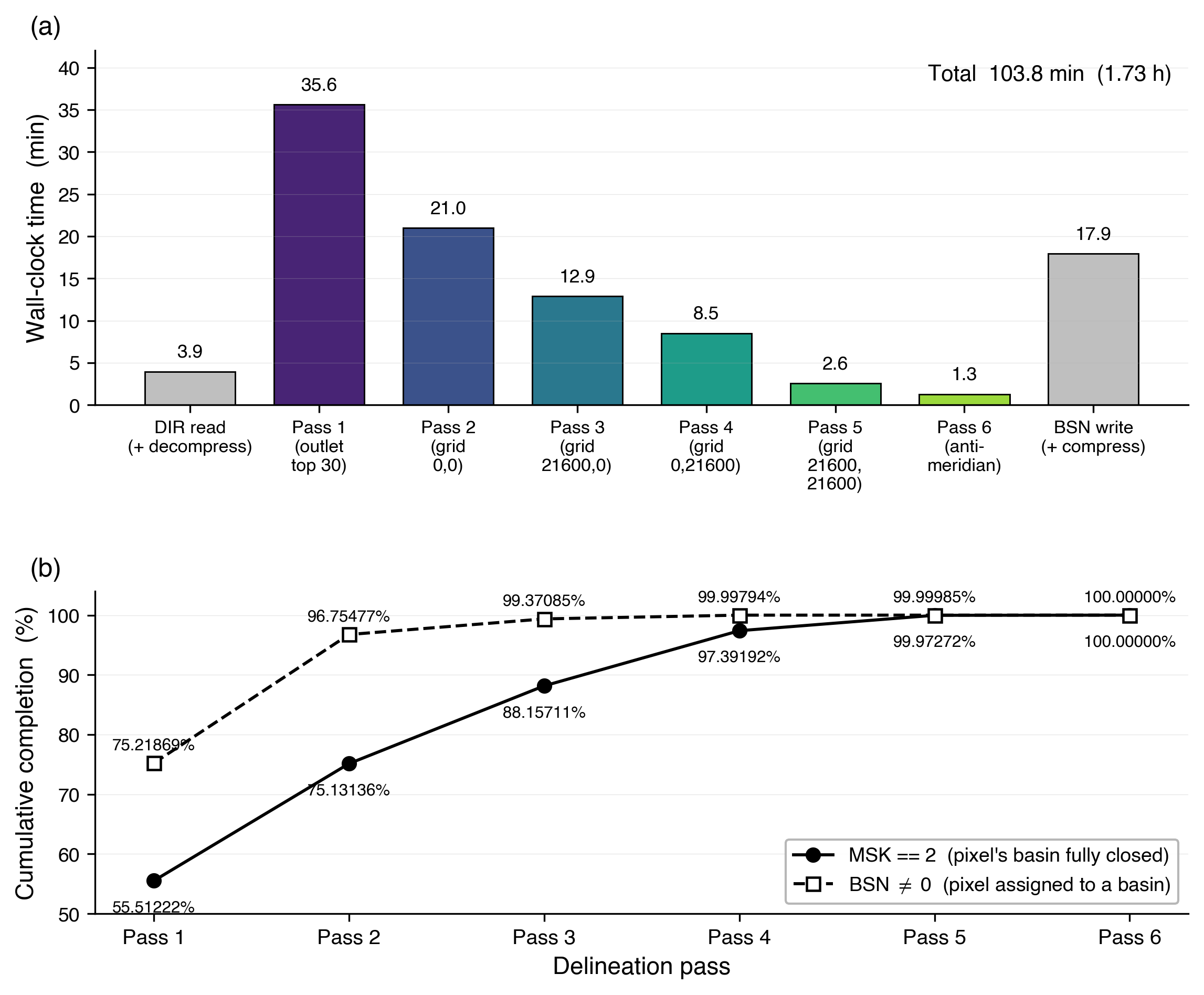
Figure A1. Wall-clock performance of the multi-pass global basin delineation on the MERIT Hydro 3 arcsec flow-direction grid (432,000 × 174,000 pixels; 22.26 billion valid land pixels; 24.59 million outlets). (a) Per-stage time: DIR GeoTIFF read, the six delineation passes (one outlet-centered tile sweep over the 30 largest basins, four offset grid sweeps, and a final antimeridian-wrap pass), and BSN GeoTIFF write. Total end-to-end wall-clock is 103.8 min (1.73 h); both I/O bars include (de)compression, not only raw disk transfer. (b) Cumulative completion after each pass: MSK == 2 (a pixel’s basin is fully closed, solid line) and BSN ≠ 0 (a pixel has been assigned a basin ID, dashed line). The two curves converge to 100 % by Pass 6; the early gap between BSN ≠ 0 and MSK == 2 reflects pixels that carry a basin ID before their basin’s traversal completes.
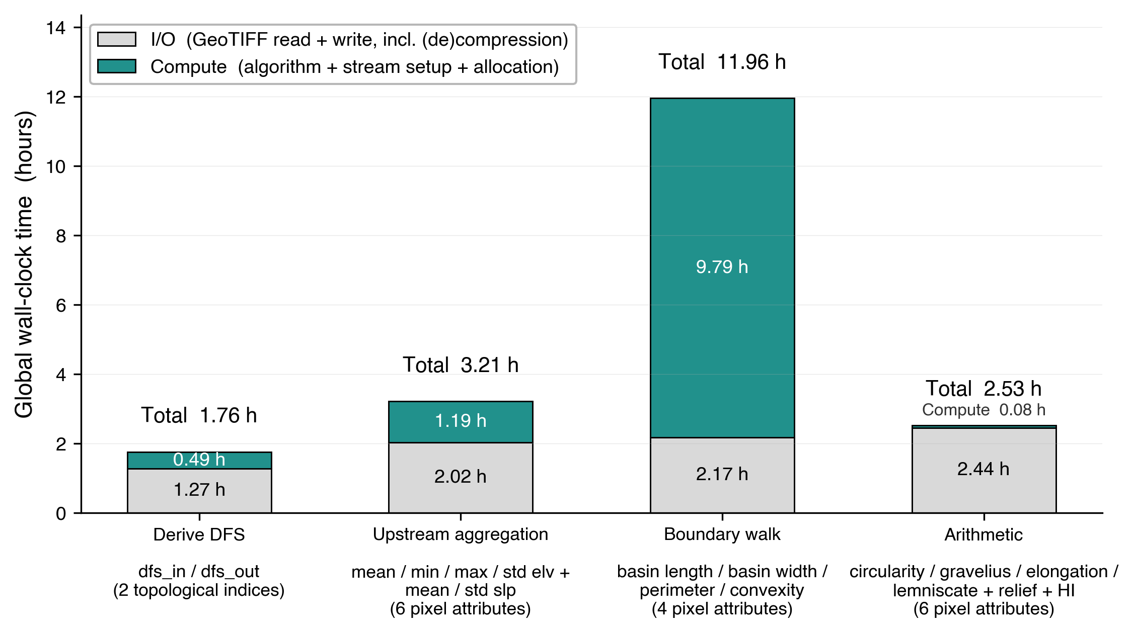
Figure A2. Global wall-clock time for each of the four computational kernels of the FullBasin pipeline. Each bar is stacked into I/O (GeoTIFF read + write, including (de)compression) and Compute (algorithm core and per-tile setup). Kernel outputs are: Derive DFS: dfs_in, dfs_out (2 pixel layers); Upstream aggregation: mean, min, max, std elevation and mean, std slope (6 pixel attributes); Boundary walk: basin length, basin width, perimeter, convexity (4 pixel attributes); Arithmetic: circularity ratio, Gravelius compactness, elongation ratio, lemniscate ratio, basin relief, hypsometric integral (6 pixel attributes). Boundary walk dominates the per-pixel attribute wall-clock at 11.96 h (~68 % of the 17.7 h spent on the 16 attribute layers), driven by compute rather than I/O; the other three kernels are I/O-bound and lie within a factor of two of each other.
Figure A3. Obtaining dfs_in and dfs_out from the released seq_dfs and the upg of MERIT Hydro, on the 8 × 8 example of Fig. 4. (a) seq_dfs (released): the dfs_in order reversed within each basin, so that the outlet holds the largest number b of its basin; at T₁, 37. (b) upg (MERIT Hydro; the pixel itself included); at T₁, 20. (c) dfs_in = a + b − seq_dfs, where b is seq_dfs at the outlet and a = b − upg(outlet) + 1; Basin A spans [0, 40] and Basin B [41, 51]; at T₁, 0 + 40 − 37 = 3. (d) dfs_out = dfs_in + upg − 1, the largest dfs_in among the pixels upstream, the pixel included; at T₁, 3 + 20 − 1 = 22. Basins occupy contiguous blocks [a, b] in the order of their outlet pixels in the tile (row by row). Intervals are closed and include the pixel itself. Light yellow marks the 20 pixels upstream of T₁; red triangles mark the outlets.
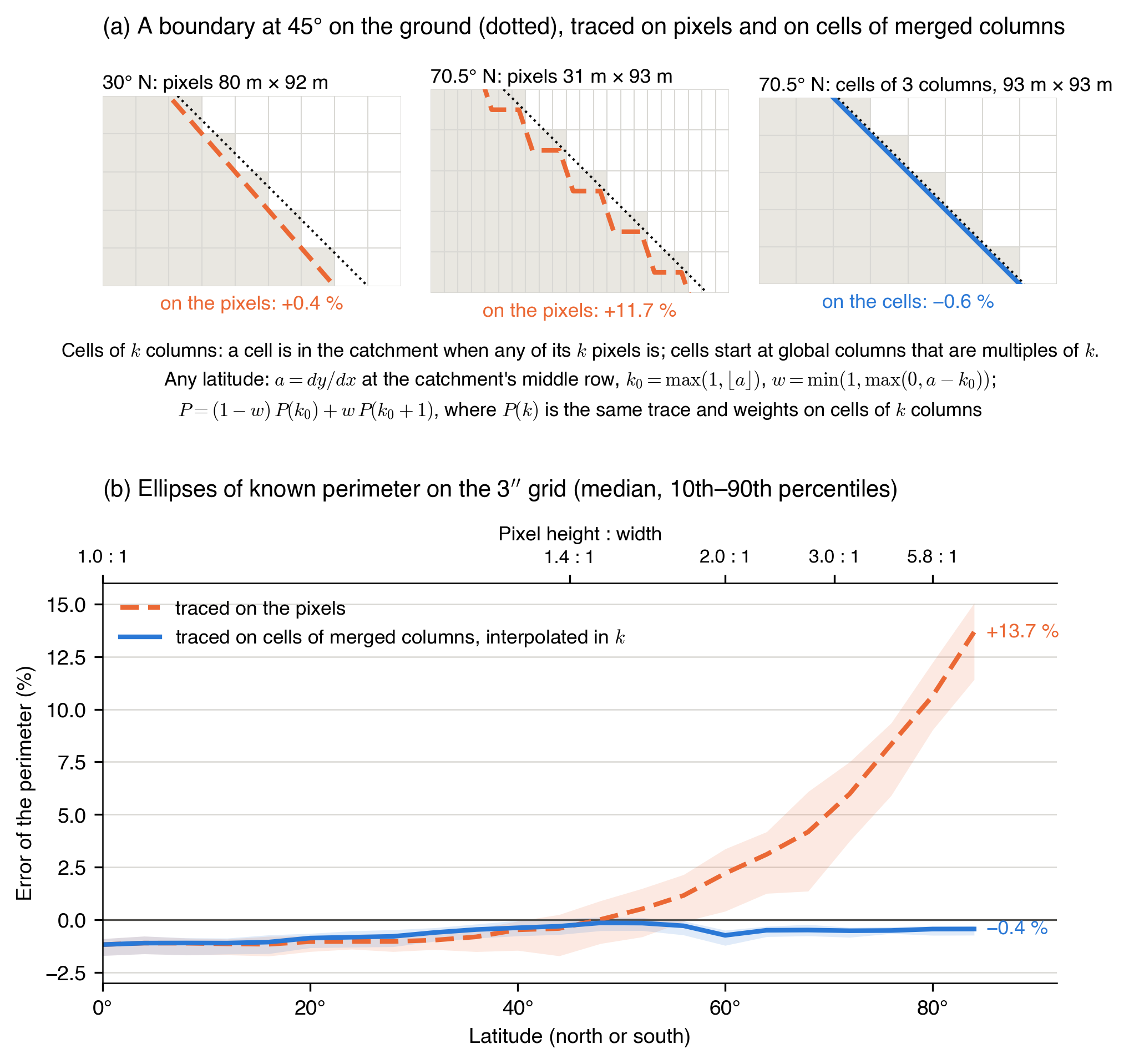
Figure A4. Extension and validation of the perimeter method. (a) A boundary at 45° on the ground, traced on pixels at 30° N (80 m × 92 m): +0.4 %; on pixels at 70.5° N (31 m × 93 m): +11.7 %; and on cells of 3 merged columns at 70.5° N (93 m × 93 m): −0.6 %. A cell of k columns belongs to the catchment if any of its pixels does; cells start at global columns that are multiples of k. With a = dy/dx at the middle row, k0 = max(1, ⌊a⌋) and w = min(1, max(0, a − k0)), the perimeter is P = (1 − w) P(k0) + wP(k0 + 1), both traced with the same tracing and weights; a ≈ 3 at 70.54° N, and a ≤ 1 within 6.59° of the equator. (b) Error against the exact perimeter for 1,320 ellipses, 60 at each latitude from 0° to 84° in steps of 4°, with semi-major axes of 30–60 pixels, axis ratios of 0.4–1, and random orientation and position; the exact perimeter is from Ramanujan’s approximation. Lines show the median and shading the 10–90 % range. On pixels the error grows to +13.7 % at 84°; on merged cells with interpolation it is −0.4 % at 84°, with medians from −1.2 % to −0.1 % across latitudes. Tracing and weights are those of the original method (Appendix B).